
PredictionDB – A Shop Window, a Filing Cabinet and 96 GB of Index Cards
The mole puts its week-ahead power price forecast on the surface for everyone, writes 110 software requirements without being forced to, and finds out that the index of its storage is bigger than the raw data.
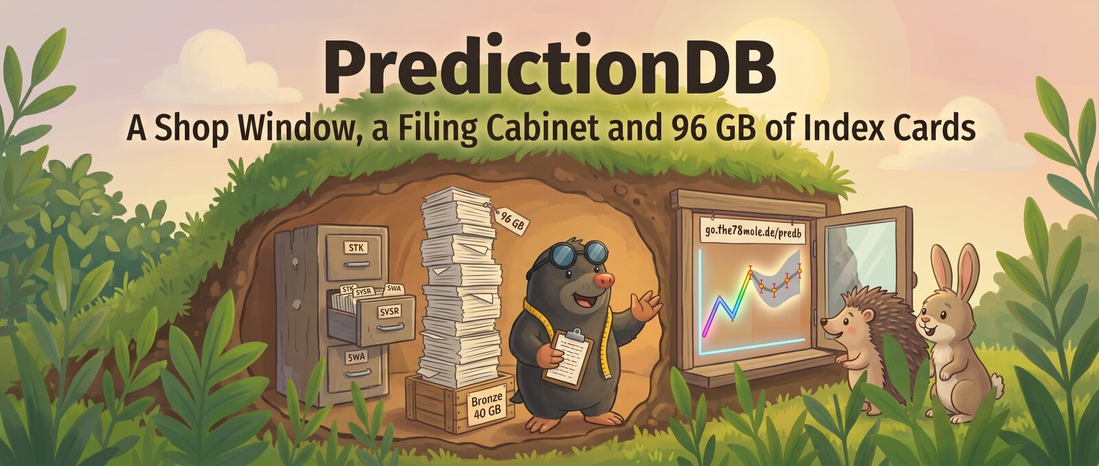
There comes a point in every mole's life when it stops digging long enough to look at what it has built – and realises it has no idea how big the burrow actually is, nobody outside can see any of it, and the only documentation is a pile of muddy notes on the tunnel walls.
That point was this week.
Previously, underground: PredictionDB forecasts German grid load and day-ahead power prices for the coming week, from free data only. Two days later it pulled three years of weather history through GitHub Actions and tripped over the clock change. Two days after that, a Thursday at 560 €/MWh taught all five model versions humility, and the burrow gained a 31-member weather ensemble.
Since then: 34 more merged PRs (#177 to #210). Fewer than last time, because some of them were the kind of work moles don't usually admit to doing. Paperwork, for instance.
| Tunnel | What happened | PRs |
|---|---|---|
| Shop window | Public week-ahead forecast with a fixed short link, daily | #195–#198, #200, #201 |
| Filing cabinet | Requirements from stakeholder down to the function, traceable in code | #193, #194, #203–#205 |
| Measuring the burrow | Storage per weather group, bronze clean-up, a tired disk | #192, #202, #206–#210 |
| Weather for all of Europe | GFS Europe gold per bidding zone, GEFS catching up | #180, #185–#191 |
| Thinking about GPUs | What training in the cloud would cost, and how the backtest works | #181, #182, #184 |
The Shop Window: A Forecast You Can Actually Look At
Three posts in, a fair question from surface-dwellers was: "Nice charts. Can I see the forecast?" Until now the honest answer was "only if you're in my basement". The Grafana runs inside the home lab, behind a login, and I'm not putting a database with my whole infrastructure on the internet just to show a line chart.
The solution (#197) is a small service that does the moley thing: it comes up for air once a day, takes a picture, and goes back down. Every day at 14:30 local time – after the day-ahead auction has published tomorrow's prices – it uploads the week panels as an interactive Grafana snapshot to snapshots.raintank.io and points a fixed short link at the newest one:
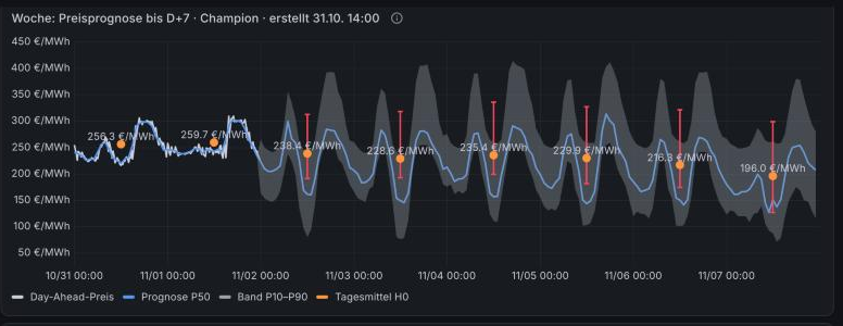
Screenshot of the public snapshot from 31 October 2026, 14:00 run. Prices: Bundesnetzagentur | SMARD.de, CC BY 4.0; forecasts from PredictionDB. The snapshot has its own panel with all sources and licenses.
What you see there:
- Load and price up to D+7 for the champion model, with the P50 as a line and the P10–P90 band in grey (#195). For each hour, the newest run that covers it wins.
- A daily mean per delivery day with a red error bar from P10 to P90 (#196). It's not the plain average: it's weighted with the BDEW household load profile H0, because a household doesn't use power evenly across the day. That's the number that matters if you're on a dynamic tariff – or if you're a mole deciding whether to charge the car this week or next.
- Today and tomorrow are real prices, not forecasts, as soon as the auction result is in.
- A list of older snapshots at the bottom, so you can check last week's forecast against what actually happened. Snapshots live for 30 days.
You can see in the screenshot what the model thinks of the next week: around 230 €/MWh, slowly easing towards 196 at the end. And you can see the band, which goes from "fairly sure" for tomorrow to "I'm a mole, not a prophet" by D+5. That band is honest. After last Thursday I'd rather show a wide band than a confident line.
Why a snapshot and not a public dashboard (click to expand)
A Grafana snapshot is a frozen copy of the panels with their data – no database connection, no live queries, nothing that can reach back into the burrow. That's exactly what I want for something public: the home-lab Grafana stays behind its login, and the internet gets a picture that happens to be interactive (zoom, tooltips, legend toggles).
The catch: raintank's snapshot server only knows Grafana's standard panels. Internally, the price panels now use ECharts for the bold daily-mean labels and the error bars (#198), so there's a separate "public" dashboard template built only from standard panels. The internal dashboard "Prognose aktuell" also moved into its own dashboard, because Grafana silently ignores relative panel time overrides as soon as you zoom once – and then your "next seven days" panel happily shows last Tuesday.
One bug surfaced right after the shop opened. Between 13:00 and the moment the auction result actually lands in the database, the model believed tomorrow's price was already known (that's the rule), found nothing there, and produced a price forecast of NaN – an empty shop window. #199 caps "known until" at the last value that's actually present, and the predictor refuses to write NaN at all. Customers prefer goods.
The Filing Cabinet: 110 Requirements, Voluntarily
Here's a confession that will make some readers question everything they thought they knew about moles: I wrote requirements. Not because a customer demanded them. Because after 200 PRs, the specification and the architecture document had started telling slightly different stories, and "the code is the documentation" stops being funny once the Compose file lists 25 services.
So #193 turned the project into a StrictDoc project under reqs/, structured along ISO/IEC/IEEE 29148, 15288 and 12207. Yes, for a hobby project. I know.
| Level | Prefix | Count |
|---|---|---|
| Stakeholder requirements (mission and guiding principles) | STK- | 25 |
| System requirements (incl. VM, Garage, Postgres, Grafana, Actions, GHCR) | SYSR- | 42 |
| System architecture | SYSA- | 28 |
| Software requirements for wx-ingest, wx-process, wx-exchange, energy-ingest, mastr-ingest | SWR-<service>- | 18 + 21 + 23 + 31 + 17 = 110 |
| Software architecture for the same five services | SWA-<service>- | 76 |
The fun part is the bottom of the pyramid. Every module points to its architecture component in the docstring, every function and test to the requirement it fulfils:
def assemble(model, resolution, run, decoded, attrs=None) -> Dataset:
    """Setzt dekodierte Schritte zu einem Datensatz zusammen (Intervallwerte siehe decode).

    @relation(SWR-WXP-012, scope=function)
    """
(Shortened from wx_process/silver.py. The docstrings are German, like the rest of the project – the mole only blogs in English.)
A pre-commit hook (reqs-abdeckung) then complains about every requirement that's marked as implemented but has no reference from the code – or, if its verification method is "Test", no reference from a test. StrictDoc itself refuses to build if anything points at an ID that doesn't exist. The rendered HTML hangs off every CI run as an artifact. Only docstrings changed in the code; the mole remains a mole.
Five services are done: wx-ingest as the template, then wx-process, wx-exchange, energy-ingest and mastr-ingest (#194, #203–#205). The ML side is still waiting for its turn at the filing cabinet. The requirements were collected afterwards from the specification, the architecture, the code and the decisions in the PRs – which is the honest way of saying the paperwork came after the tunnel. As it always does.
Measuring the Burrow
Next surprise: I didn't actually know how big everything was. So now a service measures it every hour and Grafana shows the storage per weather group – GFS Germany, GFS Europe, GEFS and "other" – split into bronze, silver, gold and metadata (#207).
The first measurement on the VM:
| What | Size |
|---|---|
| Silver (Zarr stores in Garage) | 228 GB in 1.58 million objects |
| Bronze (raw GRIB in Garage) | 40 GB |
Gold (feat.nwp_value in TimescaleDB) | 23 GB |
| Garage metadata (LMDB plus two snapshots) | 96 GB |
Read the last line twice. The object store's own index is more than twice as big as all the raw weather data. 1.58 million small objects are 1.58 million index cards, and Garage keeps them very carefully. A mole with a 96 GB card index for a 268 GB cellar – that's the kind of thing you only find out when you measure. The listing itself was slow enough that the measurement service went through three iterations in two days: list silver first and in parallel, extrapolate the rest, and finally take the months from the database instead of listing prefixes at all (#208–#210).
Two clean-ups followed. Old GFS bronze is now deleted after 92 days – but only for runs whose silver exists (#192, #206). Silver stays; I decided not to delete that.
And the disk got a break (#202). The VM's Docker disk was 100 % busy at about 980 write IOPS, but only 27 MB/s and 48 ms per IO, while the CPU was idling at 1 %. The gold writers were mostly waiting for the write-ahead log. 581 of 3,072 checkpoints were forced because max_wal_size was 1 GB. Now Postgres gets 8 GB of WAL, 15-minute checkpoints, zstd WAL compression and 64 MB WAL buffers, and only the bulk weather writers run with synchronous_commit=off. If the VM crashes, they lose the last few seconds and simply redo those runs. Everything else still commits synchronously.
What synchronous_commit=off actually risks (click to expand)
With the default, Postgres only reports a COMMIT as done once the WAL record is flushed to disk. With synchronous_commit=off it reports success right away and flushes a moment later (at most three times the WAL writer delay). The database never becomes inconsistent – a crash just loses the transactions from the last fraction of a second, as if they had never happened. For a weather job that writes features for a run and marks the run as done in the same transaction, that's harmless: after a crash, the run is simply due again. For anything a human typed in, I'd never do it.
Weather for All of Europe
The European GFS at 0.5° from the last post was collecting silver but no gold, because gold needs regions and there was no plant clustering on that grid. #190 gives it the same regions as the GEFS ensemble: 50 bidding zones as areas plus Germany's wind and PV weighted by the plant register, all under the same codes. Now GFS and GEFS can be compared zone by zone – the deterministic run against the ensemble mean and spread.
The rest of the weather work was the unglamorous kind that keeps a burrow standing: GEFS gold percentiles vectorised, backlogs worked off without pauses, blocking work moved into its own thread pool, and an import from GHCR that survives Garage timeouts (#180, #185–#189, #191). The weather dashboard now also says which service does what, because "wx-process-backfill-eu" isn't self-explanatory even to the mole that named it (#177).
Side Tunnel: What Would a GPU Cost?
LightGBM is the baseline, and the roadmap has neural networks (TFT, TiDE, N-HiTS) that have to beat it. cloud-gpu-training (#181, #184) estimated what renting the hardware would cost:
| Model | Backtest on the VM | On a rented RTX 4090 | Per month, weekly retraining |
|---|---|---|---|
| LightGBM | 3.8 h | 30–45 min (mostly more CPU cores), ~0.15 $ | ~0.60 $ |
| N-HiTS, TiDE | hours to half a day | ~1 h, under 0.30 $ | ~1 $ each |
| TFT | several days | 6–12 h, 1–2 $ | 5–8 $ |
The data isn't the problem: a training snapshot is 140 MB today, maybe 0.5–0.7 GB with the European weather and the ensemble, and it would travel through GHCR like everything else. The slowest step is exporting the snapshot on the VM (1.2–1.5 h), and that doesn't move to the cloud. The verdict for a mole on a budget: a TFT experiment costs less than a coffee, so cost isn't the excuse anymore. Time is.
To make sure the mole understands its own scoring system before it starts paying for GPUs, there's now a detailed docs/BACKTEST.md (#182) with seven Mermaid diagrams: expanding-window folds, out-of-fold stages, calibration per fold, metrics and the champion/challenger rule.
What's Next
- Results of the ablations from the last post (marginal-cost index, calibrated bands) – the mole promised not to claim anything before the backtest speaks.
- Requirements for
ml-train, the last big service without a place in the filing cabinet. - Watching the public forecast against reality. The snapshot archive makes every miss public. That's the point.
- A first neural network on a rented GPU, now that it costs less than the snacks for the evening.
The code is still on GitHub under the Business Source License 1.1, which allows internal use; check the license before you build a business on it. The data artifacts on GHCR are CC BY 4.0, with the source attributions passed on.
Back underground – but with a window now. If you walk past go.the78mole.de/predb in the afternoon, wave. The mole will be the one squinting at the error bars.