
PredictionDB – Two Days, Fifty PRs Later
Three years of weather history in about two hours, a model that got tripped up by the clock change, and a pile of side tunnels – the first follow-up from the PredictionDB burrow.
Two days ago I wrote about PredictionDB: a half-built stack that turns free NOAA weather runs and free German energy data into a week-ahead forecast of grid load and day-ahead prices. The short version: LightGBM in two stages, quantile bands, strict "what did we know at 08 UTC?" bookkeeping, and the honest admission that the price model didn't see any weather yet, because the weather history only went back to January 2026.
Then I went back underground. Two days, 51 PRs opened and 47 merged later (#59 to #111 – "fifty" is a mole rounding up), the weather history problem is mostly solved, the model has been caught tripping over the clock change, and there are four new side tunnels. Here's what came out of the dirt.
| Area | What changed | PRs |
|---|---|---|
| Weather history | GFS archive built on GitHub Actions, shipped as OCI artifacts via GHCR | #101, #102, #107, #105, #108 |
| Model | Load lags in local time across the clock change | #106 |
| Dashboards | Own forecast vs. TSO, error in %, map dashboard, champion and challenger side by side | #59, #61, #86, #89, #90, #93, #94, #96 |
| Data sources | Gas storage, LNG, oil, coal, EIA outlook, daily revision run | #79, #80, #83, #88, #97, #99, #100 |
| Analyses | Price level, futures, electrification, §14a | #78, #80, #92, #95, #98 |
Three Years of Weather in About Two Hours
The model needs weather to know whether next Thursday will be windy, and it needs years of weather to learn what that means. The GFS archive on AWS goes back to GFS v16 (March 2021), so the data is there. Getting it into the burrow was the problem.
Why the VM couldn't do it
GFS doesn't let you download a small box around Germany from the archive. You fetch byte ranges of global GRIB fields, and only about 0.4 % of what comes down the pipe is actually inside my crop. Per run that's roughly 3.3 GB of transfer for about 13 MB of silver – the compressed Zarr store that the rest of the stack works with.
My home-lab VM sits behind a line that is throttled to 8.3 MB/s. That makes it at least 6–7 minutes per run. Three years of just the 00Z and 12Z runs are about 2,200 runs, which works out to roughly ten days of non-stop downloading. The whole archive since 2021 would be around 8,000 runs, or 27 TB and 27 million range requests against AWS. That's not a tunnel, that's a mining operation.
Let the runners dig
So the digging moved to where the bandwidth is: GitHub Actions. The new workflow gfs-history.yml (#101) does this:
- A plan job reads what's already published and builds a matrix of only the months that still have gaps.
- Each matrix job handles one month of one run hour (say, September 2026, 00Z). At most 8 jobs run in parallel, each with two runs in flight. Bronze (the raw GRIB) only ever exists on the runner.
- The runner builds the silver Zarr store and pushes it to the GitHub Container Registry as an OCI artifact: one manifest per month and run hour, one layer per run, tagged like
2026-10-00z. - The VM runs
wx-exchange gfs import, pulls only the 13 MB stores it's missing, and computes the gold-tier features locally from them.
The order matters, because I want to start training as early as possible. The workflow goes in three-year blocks from the newest month backwards. Inside a block it does all 00Z runs first, then 12Z, then 06Z and 18Z. #107 taught the importer on the VM to use the same order – before that it went month by month and fetched 12Z before 00Z, which made three years of 00Z take about twice as long.
| VM over the throttled line | GitHub Actions | |
|---|---|---|
| Transfer per run | ~3.3 GB | ~3.3 GB (on the runner) |
| What reaches the VM | 3.3 GB | ~13 MB of silver |
| Three years of 00Z (36 months) | about 5 days | 2 h 09 min |
| Three years, all four run hours | about 7¾ h |
Those runner numbers come from the first real run of the workflow: the 36 jobs for three years of 00Z started at 20:28 and the last one finished at 22:37 UTC. All 144 jobs of the first block (four run hours × 36 months) were done shortly after 04:00.
OCI artifacts, ORAS and why the container registry stores weather (click to expand)
A container registry doesn't actually care whether it stores container images. Underneath, an image is just an OCI manifest – a small JSON document – pointing at layers, which are blobs addressed by their SHA-256. ORAS ("OCI Registry As Storage") is the name for using exactly that mechanism for arbitrary files. Here each layer is a tar of one run's Zarr store with its own media type, and the manifest carries annotations: the run time, a fingerprint of the inputs (variables, crop, steps, encoding version) and a content hash of the store.
Those annotations double as the state of the whole job. The plan step only has to read manifests to know which runs are missing or were built with old inputs; there's no separate database of progress. A cancelled workflow just gets started again and continues where it stopped. With rebuild, every run is rebuilt but only uploaded if its content hash changed. The client in wx-exchange talks the OCI distribution API directly and needs neither the oras CLI nor Docker. Public packages on GHCR are anonymous to read, so any other PredictionDB instance can import the same silver.
Trust, but verify
Weather built on someone else's computer should be checked. With GFS_BACKFILL_BRONZE=true the VM still downloads bronze in the background and rebuilds silver from it. Then wx-exchange gfs verify (#102) compares the local build with GHCR by content hash, without downloading the layer. Each run comes back as equal, different (with the differing chunks and attributes for the first few), imported (it's still the copy from GHCR, nothing local to compare) or local_missing. The content hash deliberately ignores the timestamp when bronze was completed, otherwise no two builds would ever match.
Watching the tunnel fill
Two new panels in the Grafana status dashboard show the progress per month as stacked bars (#105, #108): one for silver (green = present, yellow = downloading) and one for gold (green = weather features computed with the current clustering, yellow = silver is there, features still pending). A new clustering of the plant register turns everything yellow again until it's recomputed – which is exactly what should happen.
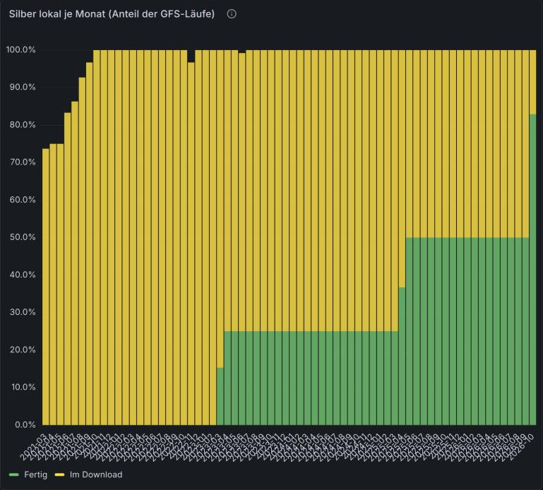
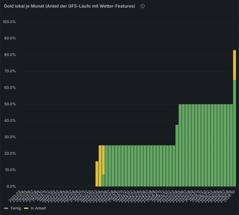
Screenshots from the PredictionDB status dashboard on 27 October 2026, all four run hours selected. Data: NOAA GFS, public domain.
Read the bars in quarters: every run hour is 25 % of a month. At the time of the screenshots, one run hour (00Z) had silver and gold from mid-2023 onwards, a second one from May 2025, and everything else was still yellow – queued on the VM, while GHCR already had it.
The honest caveats:
- The older block isn't complete. The second block (March 2021 to October 2023) was still running while I wrote this, and a few month jobs failed. In November 2022 some archived GRIB messages are missing their
7777end marker on both the AWS and Google mirrors, andgribkitrefuses truncated messages. Those runs are recorded as gaps, not papered over. - Gold is still catching up. Silver on the VM is the fast part. The weather features per plant cluster are computed by the backfill service hour by hour, and the model hasn't been retrained on the new history yet.
- Live runs still come from the VM. The workflow is for history. Publishing new runs from the VM (
wx-publish) and signing the manifests with cosign are still open.
The Mole That Got Tripped Up by the Clock Change
On Sunday, 25 October, Germany switched from summer to winter time. On Monday morning the load forecast for that day looked fine all day – except at 05:00 and 06:00 local time, where it was about 8 GW too high. The morning ramp came an hour early.
My first suspicion was the obvious one: the model doesn't know local time. Wrong. The calendar features (hour, dow, holidays …) were already computed in Europe/Berlin, and there's a daylight-saving flag on top. The culprit was further down the tunnel: the lag features. "The same hour one week ago" was implemented as ts − 7 × 24 h in UTC. Across a clock change, that's the right UTC hour and the wrong wall-clock hour.
| 26.10.2026, local time | Forecast P50 | Actual | Error | Week lag (19.10., one hour later) |
|---|---|---|---|---|
| 05:00 | 52.5 GW | 44.4 GW | +8.0 GW | 52.4 GW |
| 06:00 | 58.8 GW | 51.1 GW | +7.7 GW | 58.7 GW |
| other 22 hours | at most ±2.2 GW |
For Monday 05:00 CET, the week lag delivered the previous Monday at 06:00 CEST, and the model follows the weekly lag of the load almost one to one. The daily MAE was 1.37 GW; without those two hours it would have been about 0.8 GW.
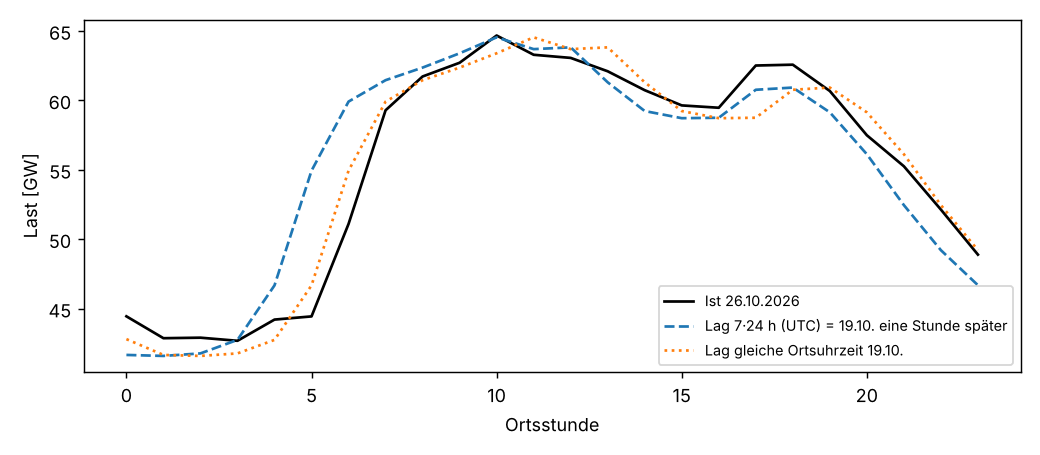
Data: Bundesnetzagentur | SMARD.de, CC BY 4.0; forecast from PredictionDB. Chart: docs/analysen/zeitumstellung.
One bad Monday is an anecdote, so I dug through every clock change since 2019 on SMARD data (8 in spring, 8 in autumn) and compared a naive "value k days earlier" forecast in both variants:
| Series | Lag | Spring: UTC → local | Gain | Autumn: UTC → local | Gain |
|---|---|---|---|---|---|
| Load | previous week | 3.58 → 3.13 GW | +12.6 % | 2.96 → 2.49 GW | +15.8 % |
| PV | previous week | 3.03 → 3.76 GW | −24.2 % | 1.40 → 1.82 GW | −30.1 % |
| Residual load | previous week | 10.36 → 10.51 GW | −1.4 % | 11.60 → 11.36 GW | +2.1 % |
| Price | previous week | 30.3 → 30.7 €/MWh | −1.3 % | 41.5 → 40.5 €/MWh | +2.4 % |
So the load lives on the wall clock – people get up at 06:00 whatever UTC says – while the sun runs on UTC, and shifting PV by an hour makes it much worse. Price and residual load are a mix of both and don't care. For the week lag of the load, local time wins in 15 of 16 clock changes (the exception is spring 2024, which collided with Easter).
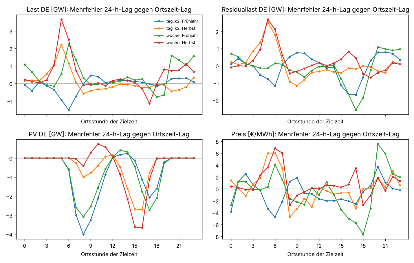
Data: Bundesnetzagentur | SMARD.de, CC BY 4.0, clock changes 2019–2026. Chart: docs/analysen/zeitumstellung.
The fix (#106) is a model config option lag_local_time. For the series listed there, the day and week lags look up the same local wall-clock time. The doubled 02:00 hour in October is averaged, the missing one in March is replaced by 03:00, and the leakage guard stays: if last week's local hour isn't published yet at issue time, the feature reaches one more week back. Both de_lu_v1 and de_lu_v2 set it for the load only. Over a whole year it barely moves the needle (−0.8 % MAE for the week lag), because only 2 of 52 weeks are affected – but in those weeks it hits exactly the expensive morning hours.
Why the daylight-saving flag didn't save me (click to expand)
The model already had a dst feature. It tells the model whether the target hour is in summer time. It doesn't tell it that the lag reaches across a clock change and is shifted by an hour. A feature like "this lag is shifted" would only be non-zero on 2 × 7 days a year – far too rare for the trees to learn to undo the shift themselves. Fixing the feature is simpler and works immediately. Existing models keep their stored config, so the fix takes effect with the next training run.
The same Monday had a second, unrelated problem: the price was off by up to −93 €/MWh at 18:00. That one was wind. The kalender variant has no weather and expected 36–37 GW of onshore wind; the afternoon delivered 16–20 GW. Which is the best argument yet for the weather history above.
Watching Our Own Forecast Against the TSOs'
Forecasts nobody looks at don't improve, so a good part of the merged PRs went into Grafana.
A fair comparison (#86). The TSOs publish their day-ahead load forecast by 10:00 local time on the day before. The new panels show, for each delivery day, only our own run issued at exactly that moment – the day before at 10:00 Europe/Berlin – next to the TSO forecast and the actual load. Same for the price against the auction result. To make that possible, ml-predict now wakes on the full hour instead of sleeping 3,600 s after each run (which drifted and skipped hours) and catches up on missed issue times after a restart.
Errors that a human can read (#59, #89). The error panels gained a second axis with the error in percent, and the info boxes now explain MAE, RMSE and that percentage in plain words.
MAE, RMSE and why the percentage isn't a MAPE (click to expand)
MAE is the average miss, regardless of direction: a forecast of 50 GW against an actual of 52 GW and one of 54 GW against 52 GW both count as 2 GW. RMSE squares the misses before averaging and takes the root at the end, so single big misses count more. RMSE is always at least the MAE; a big gap between the two means a few really bad hours rather than a generally sloppy day.
The percentage is a WAPE: the day's sum of absolute errors divided by the day's sum of absolute actual values, capped at 100 %. The usual MAPE averages the percentage error per hour, which is fine for load and useless for prices – an hour at 0.10 €/MWh or below zero blows it up to absurd values. Dividing sums instead of averaging ratios keeps a day with low prices from looking like a catastrophe.
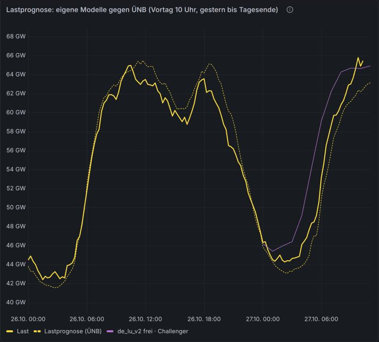
Screenshot from the PredictionDB status dashboard, 26–27 October 2026. Load and TSO forecast: Bundesnetzagentur | SMARD.de and ENTSO-E Transparency Platform, CC BY 4.0.
The first days of this panel are still thin: only the challenger has a run issued at 10:00 the day before for 27 October, because the panel and the catch-up logic only arrived on 26 October. And its morning ramp still comes early – no surprise, since the clock-change fix from above only takes effect with the next training run.
Champion and challenger side by side (#61). Last time de_lu_v2 was recommended as challenger. It turned out ml-predict only ever computed the default config de_lu_v1, so the registered challenger never produced a single forecast. Now the service runs the active versions of several model configurations in parallel and both lines show up in the panels (champion blue, challenger purple). A champion/challenger decision across configurations isn't automated yet; for now they're compared against the actuals in fcst.prediction_error.
A map (#90, #93, #94, #96). A new dashboard shows the plant clusters from the market master data register, the weather per cluster for the forecast day, and the expected energy per grid cell, split into onshore wind, offshore wind, ground-mounted and rooftop PV. Grafana's default basemap wanted an API key, the OpenStreetMap tiles had too little contrast, so the background is now a 230 KB GeoJSON of country and state borders from Natural Earth (public domain), generated by scripts/karte-umrisse.py and served by Grafana itself. And because the register knows the grid connection point of each unit, every unit now also carries its TSO control area (50Hertz, Amprion, TenneT, TransnetBW), so the map and a bar chart can split the forecast day's energy by TSO.
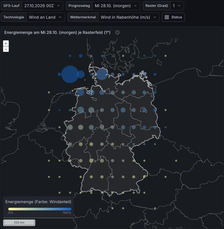
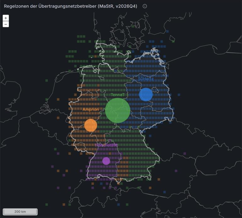
Screenshots from the PredictionDB map dashboard, 27 October 2026. Weather: NOAA GFS, public domain; plants: Marktstammdatenregister, Datenlizenz Deutschland – Namensnennung 2.0; borders: Natural Earth, public domain.
More Free Data, Still Only Free Data
The rule from the first post still holds: everything that's free and useful gets pulled in automatically through an API; anything with a restrictive license stays behind a PDB_ALLOW_* switch that defaults to off. The operator guide docs/DATENQUELLEN-ZUGANG.md lists which source needs a key and under which license it runs.
| Source | What | Key | License |
|---|---|---|---|
| GIE AGSI+ / ALSI (#79) | Gas storage per gas day (DE, AT, NL, CZ, EU), LNG terminals (DE, NL, BE, FR, EU) | free key | reuse allowed with attribution "GIE AGSI+" / "GIE ALSI" |
| Eurostat (#79, #83) | Monthly gas balance and imports by origin, crude oil import price DE, oil and hard coal balances | no | CC BY 4.0 |
| EIA Short-Term Energy Outlook (#80) | Brent and Henry Hub outlook for 0–23 months, every issue kept | no | public domain (forecasts only) |
Two details I like here. The Eurostat crude import price is the only free crude oil price I found – the Brent and WTI series at the EIA are Thomson Reuters data. And the STEO spreadsheets contain historical prices from the same vendor next to the EIA's own forecasts, so only the months after the last actual month are taken. Every issue is stored per lead month and becomes the feature group steo in de_lu_v2. Deliberately not connected: ENTSOG (no open license, automated access prohibited), Destatis GENESIS (needs an account, mostly duplicates Eurostat), and BAFA (no API, just changing PDF and xlsx links).
Data that changes after the fact (#88, #97, #99, #100). The regular sync only looked three days back, so later corrections by the sources never arrived. Now a separate service re-fetches the last 30 days once a day, remembers per dataset when it last finished (so a container restart doesn't start from scratch), and writes every changed value with old and new value into energy.value_revision. A Grafana alert reports corrections of the actual load. Its first version was too eager: Energy-Charts delivers fresh quarter hours as preliminary values and fixes them within hours – one jumped from 38.2 to 46.2 GW. Now only values that were older than 12 h when fetched count, which leaves the real SMARD corrections (for the evening of 25 October: 12 values, +1.1 to +2.6 %, arriving after about 15 h).
Side Tunnels
Four new analyses, each a script plus README with tables and charts in docs/analysen/.
What will power cost in 18 months?
preisniveau-schaetzung (#80) backtests the monthly base price 1–18 months ahead, at every first of the month from 2016 to 2026, using only data that was public on that day. The winner is almost embarrassingly simple: last month's average, shifted by the change in Henry Hub and Brent that the EIA outlook expected at the time. It beats plain "last month" by 4–7 % at 7–18 months ahead. A physical merit-order model (fuel level from the expensive hours, merit-order shape from the residual load, expected residual load from previous years) does no better than just carrying last month forward. Gas storage levels and the gas price trend don't help either – adding them makes it worse.
| Horizon (months) | STEO regression | Merit-order model | Last month | 12-month mean |
|---|---|---|---|---|
| 1–3 | 21.1 | 22.0 | 21.3 | 32.1 |
| 7–12 | 40.6 | 42.3 | 42.5 | 47.4 |
| 13–18 | 51.6 | 55.9 | 53.9 | 53.8 |
MAE in €/MWh, 130 issue dates January 2016 to October 2026.
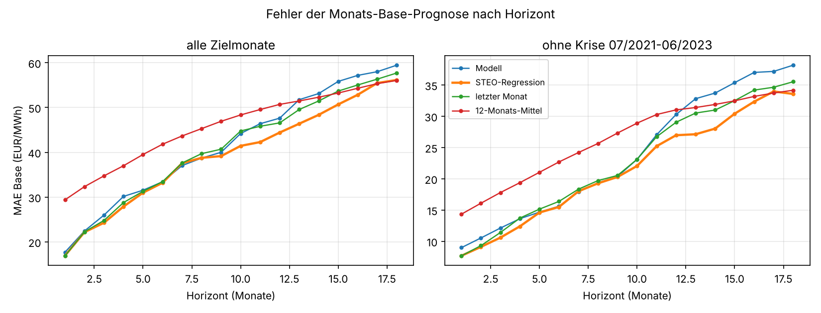
Data: Energy-Charts (Fraunhofer ISE), CC BY 4.0, prices Bundesnetzagentur | SMARD.de; EIA Short-Term Energy Outlook, public domain. Chart: docs/analysen/preisniveau-schaetzung.
The caveat is in the README too: the regression wasn't chosen blind. A first version with an intercept learned the 2016–2021 price rise as a trend and lost; only without intercept did it win. Treat 4–7 % as an upper bound.
Does the futures market know better?
There's no free source for German power futures, so I wanted to know whether I'm missing much. terminpreis-treffsicherheit (#78) compares the year-ahead base future that the TSOs use for their EEG forecasts with the spot average that actually happened, for delivery years 2017–2025. The future values were copied once, by hand, from the TSOs' public EEG publications, each row with its source; they don't go into any database or model, and nothing from the exchange is redistributed.
The result: the future did not beat a naive spot average. MAE was 72.3 €/MWh for the future, 61.4 for the spot average of the same summer weeks and 52.4 for the twelve months before. Without the crisis years 2021–2024, all three land between 8.8 and 10.5 €/MWh. The big misses happen at structural breaks, and the market misses them just as badly: in summer 2022 the future carried the peak of the gas crisis into 2023 and ended up 347 % above the actual price. Nine delivery years is a tiny sample, though – "not better than naive" holds for this period, not as a law.
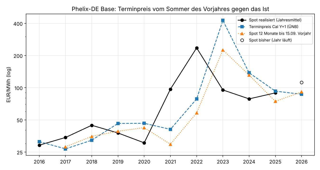
Data: futures from the TSOs' EEG publications on netztransparenz.de, transcribed by hand; spot prices Energy-Charts (Fraunhofer ISE), CC BY 4.0, Bundesnetzagentur | SMARD.de. Chart: docs/analysen/terminpreis-treffsicherheit.
What happens when everything is electric?
elektrifizierung-last (#92, #95) asks how much EVs, heat pumps and air conditioning are in the German load today, and what full electrification would do. Today the effect is small: EVs used about 5.4 TWh in 2025, household heat pumps about 8.1 TWh in 2024, together just under 3 % of 466 TWh. Air conditioning isn't visible in the load at all.
At full electrification – nearly every car electric, heat pumps wherever there's no non-fossil alternative – demand rises to about 755 TWh a year (+61 %), and the annual peak from just over 73 GW to 185 GW in a median winter and 242 GW in a cold wave like January 1997. The heat pumps set it: at −14 °C daily mean they need up to 130 GW. Smart EV charging only shaves off 15–20 GW, because a cold spell lasts days and leaves no valleys to move into.
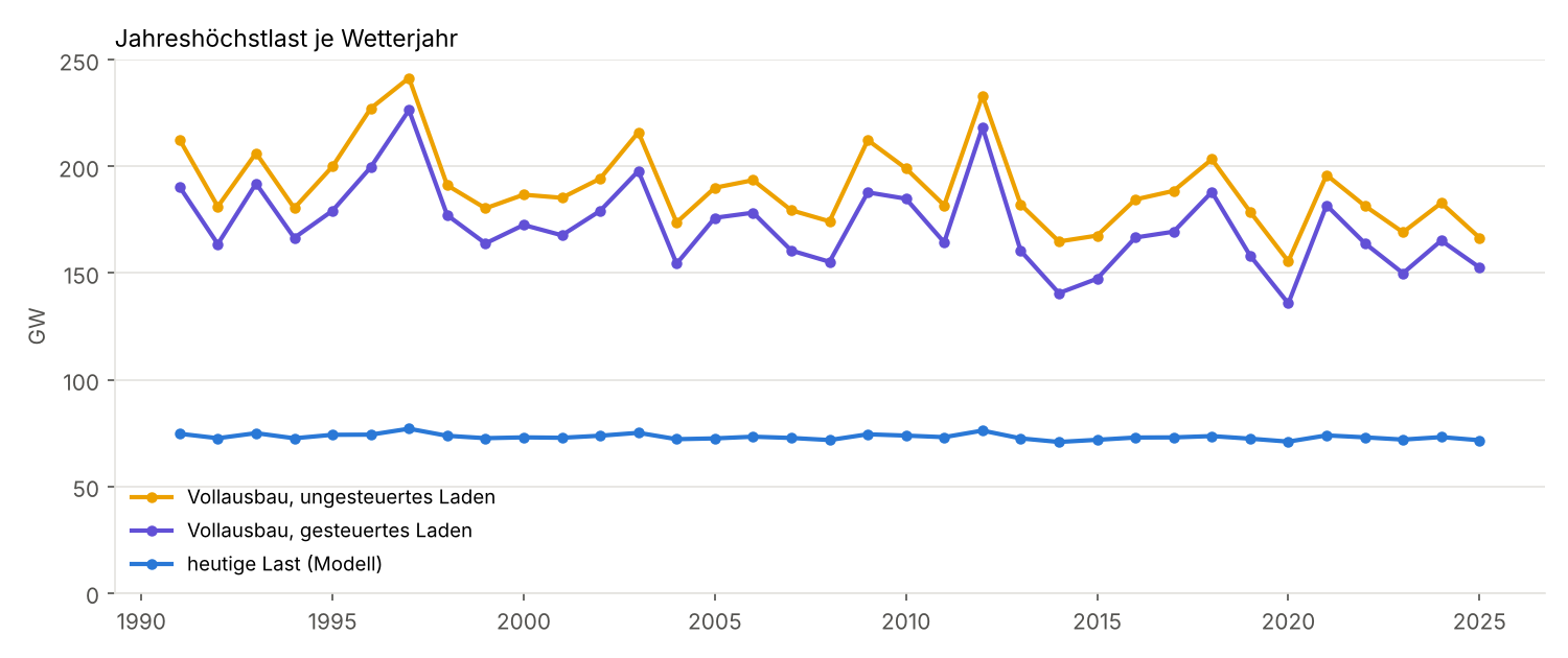
Data: load Energy-Charts (Fraunhofer ISE), CC BY 4.0; temperatures DWD Open Data, CC BY 4.0; vehicle stock Eurostat, CC BY 4.0; model and further hand-copied sources in docs/analysen/elektrifizierung-last.
Air conditioning stays a summer topic, not a peak problem: even if every second household cools, the summer peak stays at 71–72 GW, below today's winter peak. For the forecast, the useful finding is a different one: the winter load reacts more strongly to cold every year (+0.022 GW per kelvin heating degree day per year). A model trained on 2015–2020 underestimates a day with 20 K heating degrees today by about 2 GW.
Does §14a flatten the peak?
Since 2024, new heat pumps and wallboxes in Germany are "controllable consumers" under §14a EnWG, and their owners pick one of three grid-fee modules. (I dug through all 754 price sheets for that yesterday.) steuerbarkeit-14a (#98) takes a sample of twelve grid operators and the full-electrification scenario from above and asks whether module 3, the time-variable tariff, moves load out of the peak.
For the household it pays: with module 1 + 3, a wallbox saves a median €202 a year, a heat pump €205 (as an upper bound). For the national peak it does almost nothing. The high-tariff windows target the evening peak in the local low-voltage grid, but the national peak of an electrified heating sector is a cold winter morning:
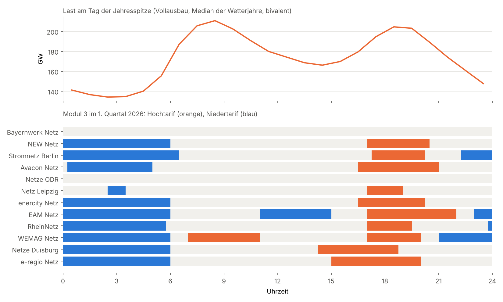
Data: grid operators' 2026 price sheets, transcribed by hand; load model as in elektrifizierung-last (Energy-Charts, DWD Open Data, CC BY 4.0). Chart: docs/analysen/steuerbarkeit-14a.
And the backup heaters push the peak up more than any control brings it down. With the bivalence point of air-source heat pumps between −5 and 0 °C, the median peak rises from 185 to 211 GW, and in a 1997-type cold wave from 242 to 312 GW – the heating rods alone draw 144 GW in that hour, while using only 8 TWh over the whole year. If all EVs in module 3 start charging when the low tariff begins, they even create a new peak at midnight (+25.8 GW). What actually helps: lower bivalence points, better insulation, heat storage, and a signal that reflects national scarcity instead of fixed local windows.
Housekeeping
- Renovate groups minor and patch updates per ecosystem and merges them itself once CI is green; majors and the Python runtime still wait for a human (#66, #70).
- CodeRabbit reviews PRs in German, skips Renovate and generated analysis output, and never blocks a merge (#73).
- Python is pinned to 3.14 (#85): the eccodes wheels only exist up to cp314, so the 3.15 update stays red until they catch up.
- CI runs on
ubuntu-26.04instead ofubuntu-latest(#103). - An optional control UI exists only as a concept in
docs/STEUER-UI.md(#60, #63). One decision is already fixed: non-free sources can only be enabled through environment variables; a UI may only switch them off.
What's Next
- Backtest the v2 weather variant on the new history – the thing the last post called the biggest lever left.
- Weekly retraining and publishing models on GHCR only once there are at least three years of GFS training data. Not before.
- Calibrate the quantile bands, which still hold 66–75 % of the actuals instead of 80 %.
- Analog and recency features only after the plain LightGBM has proven itself with weather.
The code is still on GitHub under the Business Source License 1.1, which allows internal use; check the license before you build a business on it. The data artifacts on GHCR are CC BY 4.0, with the source attributions passed on.
Back down the tunnel. Somewhere in those three years of weather the model is about to learn what a windless Monday in October looks like – and this time, at the right hour.