
PredictionDB – Sixty-Seven PRs and One Very Expensive Thursday
The forecast met a 560 €/MWh evening and lost. Meanwhile the burrow learned to read a weather archive without a table of contents, got a 31-member ensemble, calibrated bands and a merit order built from the plant register.

Every mole knows the feeling. You come back to the burrow, proud of the tunnel you dug yesterday, and find that the ceiling has quietly come down on it.
Two days ago I wrote about three years of weather history in two hours, and before that about why a week-ahead power price forecast is worth having. Short recap for anyone who just surfaced: PredictionDB forecasts German grid load and day-ahead prices for D+1 to D+7 from free data only – NOAA weather runs, SMARD, Energy-Charts, the plant register – with a two-stage LightGBM and quantile bands.
Then came Thursday, 29 October 2026, and the day-ahead auction said: 314.8 €/MWh on average, 560 €/MWh at 17:00. Every single one of my five active model versions was too low. In every single hour. This post is about that Thursday, about what the 67 merged PRs since the last post (#110 to #176) dug up, and about how a mole learns humility from a price curve.
| Tunnel | What happened | PRs |
|---|---|---|
| The expensive Thursday | Post-mortem, marginal-cost index, merit order from the plant register | #130, #144–#146, #149 |
| Weather before 2021 | GFS v15 from the NCAR archive – tooling built, backfill paused | #116–#138, #147, #160 |
| Weather, but 31 times | GEFS ensemble and GFS at 0.5° for the whole European grid | #167, #168, #170, #172–#175 |
| Honest bands | Calibration per lead day, rotating issue hours, rest-of-today D+0 | #166 |
| The neighbours | Cross-border trade and flows, neighbours' load forecasts | #159, #165 |
| Dashboards | Split in three, today and tomorrow with all forecasts D+1 to D+7 | #129, #133, #158, #161, #171 |
| Side tunnels | Batteries, energy sharing, intraday | #150, #152, #156, #162 |
The Thursday That Wasn't in the Training Data
Here's the crime scene. The black line is what the auction delivered. The coloured lines are my models, all issued on Wednesday at 08 UTC, before the auction closed:
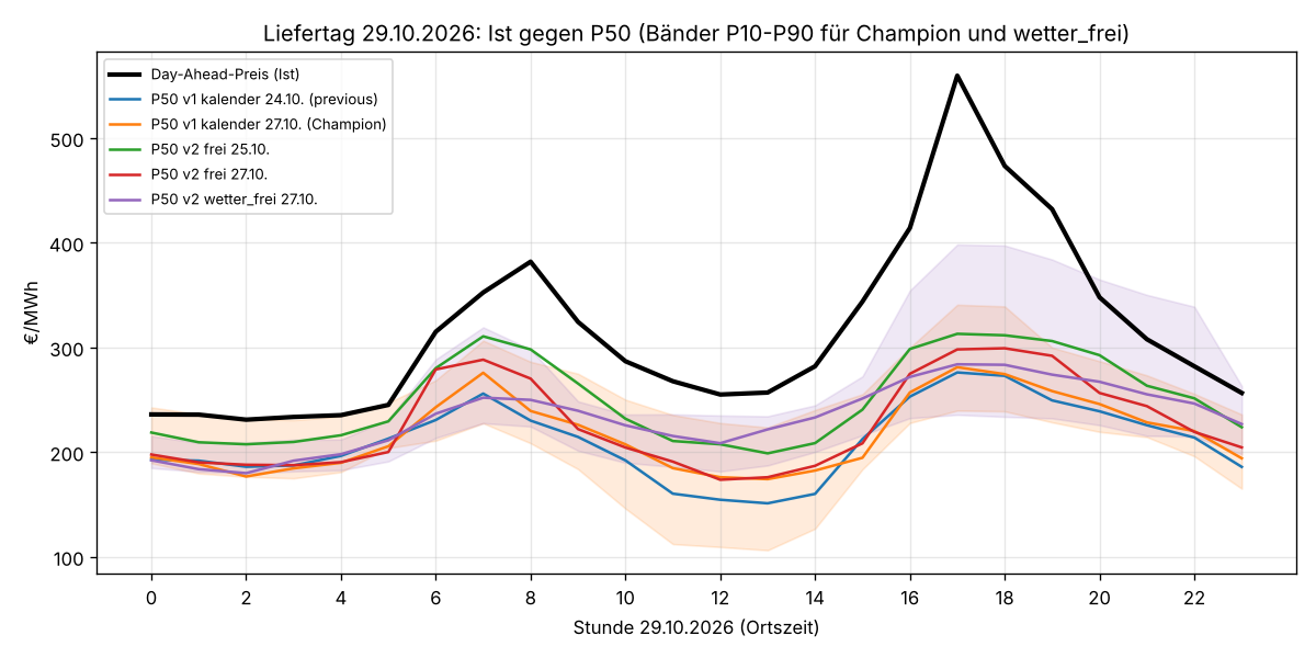
Data: day-ahead prices Energy-Charts and SMARD (Bundesnetzagentur | SMARD.de), CC BY 4.0; forecasts from PredictionDB. Chart: docs/analysen/preisabweichung-2026-10-29.
The P50 forecasts averaged between 210 and 250 €/MWh. The MAE was 65 to 105 €/MWh, and it was exactly equal to the bias – not one version was too high in any hour. The P10–P90 band, which is supposed to contain the truth 80 % of the time, managed 1 to 9 of 24 hours. The evening peak at 17:00 didn't just leave the band, it left the postcode.
The fun part: the day before, the same models were fine. For Wednesday they forecast 229 to 245 €/MWh against an actual 249 – even though that day had also jumped by 94 €/MWh from the day before. So what broke on Thursday?
Suspect 1: fossil fuel prices
The obvious suspect was guilty, but only of the level. Gas in Europe (World Bank, TTF) was 75 €/MWh in September 2026, against 32 a year earlier. Brent went from 68 to 117 $/bbl, coal from 106 to 147 $/t, and German heating oil from 0.57 to 1.15 €/l net. At the same residual load, power is now almost twice as expensive as it was from 2023 to early 2026. The night price on Thursday of 231 to 245 €/MWh is exactly what gas plants cost at that gas price.
But fuels don't explain the jump from Wednesday to Thursday. That was the wind: onshore plus offshore delivered 47 GW on 24 October and 13 GW on the 28th, and the neighbours with lots of wind went up the most (DK1 +89, CZ +51, PL +46, AT +39 €/MWh).
Suspect 2: the model's own good manners
The models were trained to be sensible, and sensible was wrong. In order of damage:
- "It'll calm down again." All price models learn relative to the last known day's average. Wednesday was twice the 7-day mean (249 vs. 121 €/MWh). After such outlier days the price fell again in 19 of 24 cases since 2018, median −24 €/MWh. The trees learned that rule perfectly and pulled Thursday's P50 down by 11 to 44 €/MWh. Thursday was one of the rare exceptions, like the dark doldrums of 11/12 December 2024 (266 → 395 €/MWh).
- Fuel prices barely register. The champion v1 has no fuel features at all. The v2 models have them, but only as monthly or weekly values with up to five weeks of delay. On Thursday they contributed +2 to +7 €/MWh. During training, the price memory (yesterday, last week) was the faster way to the price level, so the trees mostly ignored fuels. Daily gas and CO₂ prices are missing entirely.
- No weather, too much wind. v1 and v2
freiforecast 18 to 21 GW of wind for Thursday. The weather variantwetter_freiwith GFS said 8 GW and correctly saw a high residual load – but then the neighbours' prices from the day before pulled its P50 down by 57 €/MWh, the Czech average alone by 42. You can't win them all. Apparently you can't win any. - Bands too narrow anyway. In the backtest, P10–P90 covers 57 to 67 % instead of 80 %. A scarcity spike of 560 €/MWh in a windless evening was never going to fit.
The fix: measure the fuel level from the power market itself
There's no free daily gas or CO₂ price. Trading Hub Europe wants written permission for every copy, the ACER LNG assessment has a contradictory license note, and the World Bank only publishes monthly. And LightGBM can't extrapolate beyond the price levels it has seen in training. So #149 reads the fuel level straight out of the power market, from SMARD data that's already in the database:
gk_hoch_*: the median price in hours of high residual load (top quartile) over the last 14, 28 and 56 days – that's where gas or hard coal sets the price.gk_braunkohle_*: the median price in hours when lignite runs at part load and hard coal and gas are almost off. Lignite has no traded fuel price, so this tracks the CO₂ price.gk_niveau: the shortest window that has a value, at least 20 €/MWh. With the new optionscale, the price target is learned as the deviation from yesterday's mean relative to that level instead of in €/MWh. A model trained at 80 €/MWh no longer has to have seen 300 €/MWh to forecast it.
Whether that actually helps will be decided by the ablation backtest, which hadn't run yet when I wrote this. I'm not making the same mistake twice in one post.
Could I just back out the CO₂ price from power prices? (click to expand)
I tried, in eua-rueckrechnung (#146). The idea: in hours when lignite sets the price, the price is almost pure CO₂ cost. Outside the gas crisis, that estimate landed 5–9 €/t from the auction price in monthly means from 2018 to 2025; in 2022 it was 46 €/t off. Against the mandatory baseline – just carrying forward the last known EU auction price – it loses: in the test from 01/2024 to 06/2025, the carry-forward has an MAE of 8.9 €/t, the uncalibrated formula also 8.9, and every calibrated variant 9.3 to 14.0 €/t. Verdict: a plausibility check, not a data source.
The same goes for petrol station prices as a fast oil indicator (#145). The Tankerkönig API is CC BY 4.0 and a small daily sample index would be possible, but there's no free history, and the historical archive is CC BY-NC-SA, which doesn't fit a project whose models are meant to be published freely.
Building the merit order from the plant register
While I was down there anyway: what does the supply curve of the auction look like if you rebuild it from free data? The real aggregated bid curves are sold by the exchange, cost from about 68 €/month, are only for members and must not be passed on. So merit-order (#130) builds it from every combustion unit, CHP plant and storage unit in the plant register, with efficiencies by age and technology and the fuel prices of the day:
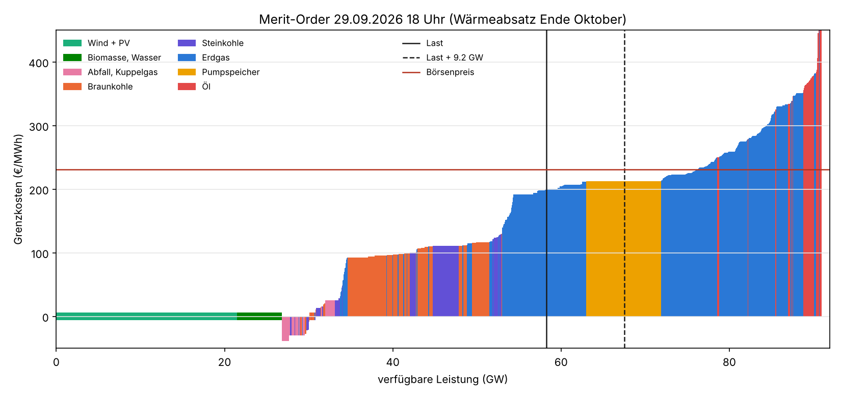
Data: Marktstammdatenregister, Datenlizenz Deutschland – Namensnennung – 2.0; prices, load and generation SMARD and Energy-Charts, CC BY 4.0; fuel prices World Bank Pink Sheet (CC BY 4.0) and EIA (public domain); EUA price for one day transcribed by hand. Chart: docs/analysen/merit-order.
The shape fits well, the level only after a fudge. Without correction, the staircase is 35 €/MWh too cheap on average over the last 30 days; adding a flat 9.25 GW to the load brings the MAE from 41.8 down to 28.3 €/MWh and the correlation from 0.86 to 0.91. Those 9 GW stand for exports to more expensive neighbours, balancing reserve that isn't offered on the spot market, plants in revision and industrial plants that only cover their own demand – and yes, the number is fitted on the same 30 days it's judged on.
The striking part is the gap: gas costs almost five times as much per unit of heat as imported coal (97 vs. 20 €/MWh), and a CO₂ price of 86 €/t only closes part of it. The moment gas sets the price, it jumps from just over 110 to almost 200 €/MWh. In the exchange price you see two plateaus: windy hours at 100–150, everything else at 190–230 €/MWh. Thursday lived on the upper plateau, with a scarcity spike on top.
Weather Before 2021: Reading an Archive Without a Table of Contents
The last post brought GFS v16 history back to March 2021. The model would love more winters than that, and the NCAR archive GDEX d084001 has GFS at 0.25° from 15 January 2015, under CC BY 4.0 (#116). There's just one catch: it has no .idx files.
What an .idx file is and why its absence hurts (click to expand)
A GRIB2 file is a long concatenation of messages, one per variable and level – a few hundred per forecast step. The .idx file next to it is the table of contents: one line per message with its byte offset. With it, you fetch exactly the 22 messages you need via HTTP range requests and ignore the rest. Without it, you either download the whole file (20–30 GB per run instead of about 1.5 GB) or you walk the file message by message, reading each header to find out what it is.
So the first version did exactly that: read the 512-byte header of every message via range request. That's about 70,000 range requests per run, each with roughly half a second of latency to the OSDF cache. The first real run took 23 minutes. A month of 30 runs would have taken around 11 hours – the job limit on GitHub Actions is 300 minutes. A mole recognises an impossible tunnel when it sees one.
What followed was a small engineering saga in nine PRs:
- More shovels (#118): 96 parallel requests per job instead of 24. Still about 9 minutes per run.
- Jump instead of walk (#120): within one model version the order of messages is fixed, only their lengths vary. So the complete inventory of a step becomes a template for the same step in later runs: estimate where the wanted message should be (scaled by file size), jump there, find the next message start, and check the header. If it's off, jump again.
- Templates in the repo (#126, #127, #128): rebuilding the templates in every workflow run kept timing out, so they now live in the repository as a 0.6 MB file – eventually 93 of 93 steps, with variants for 2019-06 to 2021-03.
- Write the table of contents once, for everybody (#135): a new workflow builds complete
.idxfiles in the exact format ofwgrib2 -s– all messages, not just my 22 – and publishes them as an OCI artifact on GHCR, one layer per month and run hour. Against real NOAA files from the AWS archive, all 4,050 lines matched. Once those exist, the history build reads the.idxfrom GHCR instead of the headers (#147). - Accepting that archives rot (#160): in March 2021, one file has 0 bytes and two are truncated, at both the cache and the origin. The job went through three retry rounds of 30 to 40 minutes each for those three files. Now they're marked
brokenand left alone.
And then, honest ending: I stopped the v15 backfill. The tooling is in place and the first tables of contents are on GHCR, but for now the training data stays with GFS v16 from March 2021. I may come back to that tunnel later. Prepared for it is a feature group nwp_version that tells the model which GFS version a run came from, because the 10 m wind has a bias jump from v15 to v16; no variant uses it yet. Meanwhile the regular v16 history workflow now runs on a daily schedule to pick up new runs from the archive by itself (#114).
Weather, but 31 Times: GEFS and a Bigger Map
A single forecast tells you what the model thinks. An ensemble tells you how sure it is – and for D+5 that's the more interesting question. GEFS runs the same model 31 times with slightly perturbed starting conditions (#167, #168, #170):
| GEFS in PredictionDB | |
|---|---|
| Members | 31 (gec00, gep01–gep30), 00Z, 6-hourly to 384 h, 0.5° |
| Variables | Temperature 2 m, wind 10 m and 100 m, precipitation, cloud cover, radiation |
| Area | 34.5–71.5° N, 10.5° W–45° E: the whole European interconnected grid incl. GB, Ireland, Nordics, Ukraine, Moldova, Turkey |
| Regions | Germany weighted by installed capacity from the plant register, plus area-weighted zones for 52 bidding zones |
| Silver | about 2.5 MB per run (members × steps × regions × variables), on GHCR |
| Gold | mean, standard deviation, P10 and P90 over the members per region |
A real test run against AWS fetched 31 × 65 files without a single failure in 157 seconds. History for completed months is built on GitHub Actions; the current month is built live on the VM, which keeps the cropped bronze (about 140 MB per run) for 183 days and only deletes it once GHCR has a silver layer with the same content.
Alongside it, GFS now also comes in a 0.5° version for the same European area (#174), loaded only from AWS and Google so that NOMADS stays free for the German high-resolution feed. Gold for that one waits for a clustering on its grid. The idea behind both: Germany's price doesn't stop at the border, so neither should the weather. Thursday's neighbours made that point rather loudly.
Bands That Admit What They Don't Know
Quantile bands that hold 57–67 % instead of 80 % are a polite way of being overconfident. #166 adds three things:
- Conformal calibration per lead day. The model is first trained without the last 12 months, the outer quantiles are measured on those months per target and lead day, the resulting shifts are stored, and then the model is trained on everything. If D+6 has earned a wider band than D+1, it gets one.
- Rotating issue hours. Day n in training uses issue hour 2, 8, 14 or 20 UTC in turn. The model sees all times of day that
ml-predictactually runs at, without more rows. - D+0, the rest of today. Already published day-ahead prices are no longer a training target and replace all quantiles in the output. There's no point forecasting what's already on SMARD.
Conformal calibration in one paragraph (click to expand)
You hold back a slice of data the model has never seen, let it predict P10 and P90 there, and count how often the truth falls outside. If P90 is exceeded 18 % of the time instead of 10 %, you shift P90 up until it's exceeded 10 % of the time on that slice – and you apply that shift to future forecasts. It makes no assumption about the shape of the error distribution, only that the future misbehaves roughly like the recent past. Thursday will test that assumption, too.
These only take effect for newly trained de_lu_v2 versions, and the backtest per lead day with calibration was still pending at the time of writing.
The Neighbours Get a Seat at the Table
#159 loads cross-border trade and physical flows per border from Energy-Charts (AT, BE, CH, CZ, DK, FR, LU, NL, NO, PL, SE plus the net sum), and the day-ahead load forecasts of eleven neighbouring zones from the free part of ENTSO-E. A live check for 27 October at 12:00 showed a net trade of −4,758 MW – Germany exporting, which happens to fit the "missing 9 GW" in the merit order. The model features follow once the history is loaded.
For weather clusters abroad, I'd need something like the German plant register in every neighbouring country. #165 checked: Switzerland, Denmark, France, the Netherlands, Belgium, Norway and Sweden have usable free registers or statistics, Austria, Czechia, Poland and Italy don't have an open register. National totals per technology come from Energy-Charts for all twelve.
Dashboards: Yesterday, Today, Tomorrow
The single status dashboard had grown into a scroll marathon, so #133 split it into three: forecasts and energy data (the new start page), weather, and system. The forecast dashboard now shows yesterday, today and tomorrow, each with the day-ahead price and every forecast that was ever made for that day – D+7 down to D+1, from the 10:00 run, for champion and challenger (#158, #161). You can watch a forecast converge as the delivery day approaches. Or, on certain Thursdays, watch them miss together.
A newly registered model version now also back-fills the issue times of the last 72 hours that the other versions already have (#129), so a challenger shows up in the comparison panels immediately instead of a day or two later.
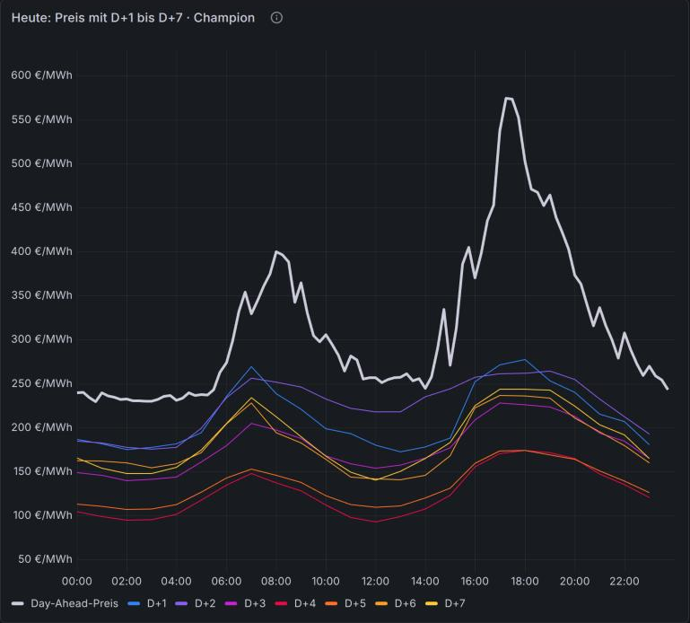
Screenshot from the PredictionDB forecast dashboard on 29 October 2026. Day-ahead price: Bundesnetzagentur | SMARD.de, CC BY 4.0; forecasts from PredictionDB.
This is the champion's view of that Thursday: seven forecasts, issued between one and seven days ahead, and every one of them below the actual price all day. The quarter-hourly price even touches 575 €/MWh around 17:00. The closer forecasts (D+1, D+2) are at least a bit closer – which is about the only good news in this picture.
Side Tunnels
When do batteries start to move the price?
batteriespeicher-preiswirkung (#150, #152) doesn't take the battery build-out from government targets but from what's actually in operation and planned in the plant register. Market-operated storage grew from 2.4 to 4.7 GW within the twelve months of the base year alone. The effect is already there: about 2 GW of extra storage cuts the average daily price spread by 10 %.
| End of | Market GW | Daily spread | Evening 17–21 | Noon 11–15 |
|---|---|---|---|---|
| 2026 | 5.1 | −6 % | −2 €/MWh | +2 €/MWh |
| 2027, build-out like 2026 | 7.5 | −14 % | −4 €/MWh | +4 €/MWh |
| 2027, register plans on time | 12.5 | −26 % | −8 €/MWh | +9 €/MWh |
| 2028, register plans on time | 17.0 | −33 % | −11 €/MWh | +13 €/MWh |
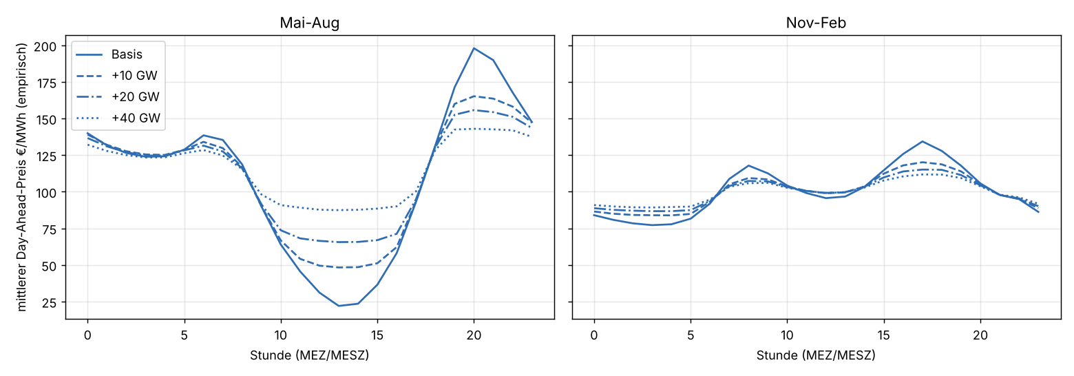
Data: Marktstammdatenregister, Datenlizenz Deutschland – Namensnennung – 2.0; prices, load and generation SMARD, CC BY 4.0. Chart: docs/analysen/batteriespeicher-preiswirkung.
Batteries smooth, they don't make power cheaper: up to 10 GW of extra storage, the average price stays within ±0.4 €/MWh. And they eat their own lunch – the pure day-ahead arbitrage revenue drops from 82 €/kW/a at 2 GW to 36 at 20 GW. For my PV battery from the first post that's a mixed message: the summer noon dip gets shallower, the evening peak lower. For the forecast model it's a warning: by 2027 it will show this as a systematic error, too low at noon and too high in the evening.
A supplement on energy sharing under §42c EnWG (#156) finds that a community of post-EEG prosumers with batteries, consumers and a wind turbine earns noticeably more in 2027, mostly because its direct marketer runs the small batteries by the exchange price – a post-EEG battery is worth about 950 instead of 630 €/kWh over 15 years. On the national price, though, it barely registers.
Can I guess the intraday price?
No, not usefully (#162). There's no free intraday price feed, so intraday-schaetzung asked how far free forecast errors explain the gap to day-ahead. The median distance is 19 €/MWh; the largest 0.1 % of quarter hours make up 65 % of the variance, and nothing free explains those. With hindsight (actual wind, PV and load) a robust model cuts the error by 8 %. Beforehand, the best model is no better than "intraday = day-ahead". Which is, if you think about it, a compliment for the day-ahead market.
Housekeeping
- Weather backfills that were orphaned by deploys get adopted instead of dying silently, and database sessions no longer pile up after a restart (#141, #148).
- The training job shows its progress in Grafana (#115), and the weather query uses bounds on
valid_timeso TimescaleDB can skip whole chunks (#140). - Price sources are synced before the slow ENTSO-E calls, so a sluggish API doesn't delay the day-ahead price (#176).
What's Next
- Ablation backtest of the marginal-cost index (
frei_gk,frei_gk_skaliert,wetter_frei_gk_skaliert) – and the calibrated bands per lead day. - Train the weather variants on the v16 history since March 2021, once the gold tier has filled up – and maybe one day resume the v15 backfill.
- GEFS spread as a feature, so the model knows on which days to be less sure of itself.
- Neighbour features from trade, flows and load forecasts once their history is loaded.
The code is still on GitHub under the Business Source License 1.1, which allows internal use; check the license before you build a business on it. The data artifacts on GHCR are CC BY 4.0, with the source attributions passed on.
Back underground. Next time the auction throws a 560 €/MWh evening at me, I'd like at least one of my models to have raised an eyebrow.